How to Make a Scatter Plot in Excel – Step by Step Guide

Curious to know how to make a scatter plot in excel? A Scatter graph is another word for the scatter plot, and they are related to line graphs. A scatter plot applies dots for the representation of data pieces. In contrast, line graphs use lines X and Y. Statistically, scatter plots are used to identify if two variables are associated in any way. For this purpose, you need to know how to do a scatter plot in Excel.

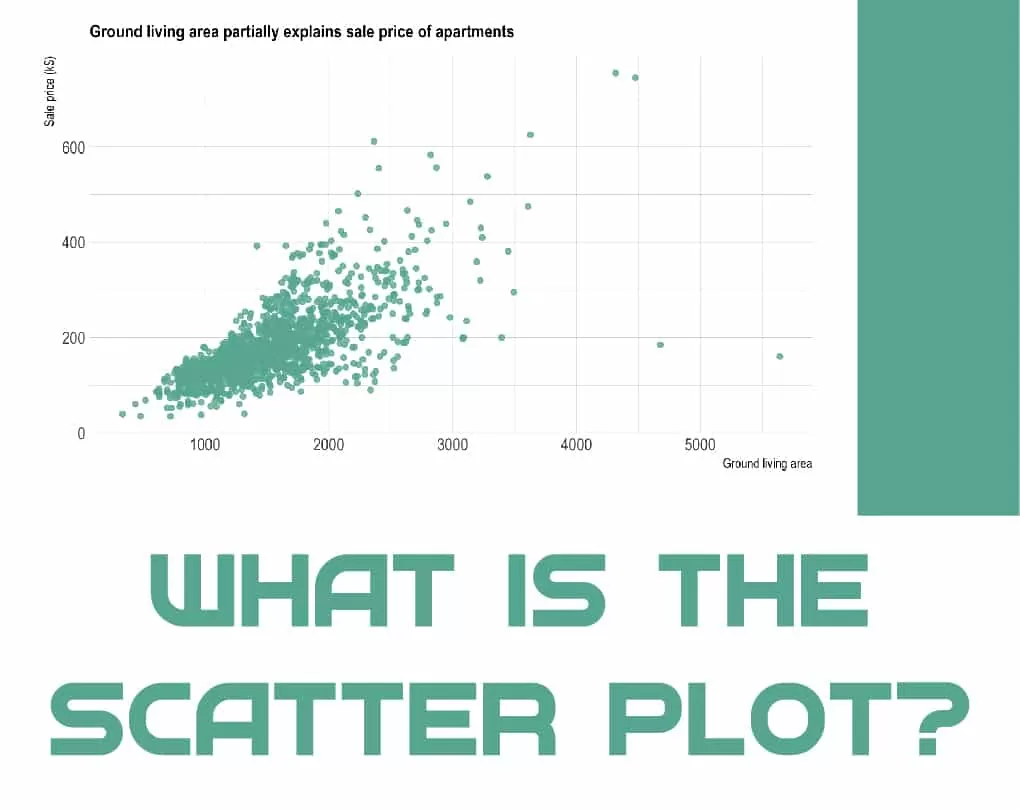
What is the Scatter Plot? 

Scatter plots (also called scatter graphs) are related to line graphs. A line graph utilizes a line on an X-Y axis to plot a continuous function, while a scatter plot utilizes dots to reproduce individual pieces of data. In statistics, these plots are helpful to see if two variables are related to each other.

For example, a scatter chart can recommend a linear relationship (i.e., a straight line). Scatter plot telling a linear relationship. Scatter plots are too named scatter graphs, scatter diagrams, scatter charts, and scattergrams.

Correlation in Scatter Plots

The relationship between variables is called Correlation. Correlation is just a different word for relationships. For example, how much you weigh is related to how much you eat. There are two kinds of Correlation: positive Correlation and negative Correlation. Suppose data points make a line from the origin from low x and y values to high x and y values the data points are positively correlated, like in the above graph. If the graph starts with high y-values and continues to low y-values, the graph is negatively correlated.

You can study positive Correlation as something that produces a positive result. For example, the more you utilize, the better your cardiovascular health. “Positive” doesn’t necessarily mean “good”! More smoking leads to more chances of cancer, and the more you drive, the more likely you are to be in a car accident.

How to Make a Scatter Plot in Excel

For example, assume that you want to look at or analyze these values. The worksheet range A1: A11 notes numbers of ads. The worksheet range B1: B11 displays the resulting sales. With this collected data, you can explore the effect of ads on sales—or the lack of an impact. To produce a scatter chart of this information, take the following steps:

1. Select the worksheet range A1: B11.
2. On the Insert tab, hit the XY (Scatter) chart command button.
3. Choose the Chart subtype that doesn’t include any lines.
4. Excel presents your data in an XY (scatter) chart.
5. Confirm the chart data organization.
6. Verify that Excel has, in fact, correctly arranged your data by looking at the chart. If you aren’t satisfied with the chart’s data design— maybe the data shows behind or flip-flopped — hit the Switch Row/Column command key on the Chart Tools Design tab. (You can even try with the Switch Row/Column command, so try it if you think it might help.) Remark that here, the data is correctly organized. The chart shows the common-sense result that raised advertising appears to connect with increased sales.
7. Annotate the chart, if appropriate.
8. Add those little fanfares to your chart that will make it more attractive and readable. For example, you can use the Chart Title and Axis Titles buttons to annotate the chart with a title and descriptions of the chart’s axes.
9. Add a trendline by hitting the Add Chart Element menu’s Trendline command key.
10. To display the Add Chart Element menu, hit the Design tab, and then hit the Add Chart Element command. For the Design tab to be displayed, you must have either first selected an embedded chart object or showed a chart sheet.
11. Excel displays the Trendline menu. Select the type of trendline or regression calculation you want by clicking one of the trendline options. For instance, to make simple linear regression, click the linear button. In 2007 Excel, you compute a trendline by ticking the Chart Tools Layout tab’s Trendline command.
12. Add the Regression Equation to the scatter plot.
13. To determine the equation for the trendline that the scatter plot uses, prefer the More Trendline Options command from the Trendline menu.
14. Then select both the Display Equation on Chart and the Display R-Squared Value on Chart checkboxes. This instructs Excel to add the simple regression analysis data necessary for a trendline to your chart. Note that you may need to scroll down the pane to see these checkboxes. In Excel 2007 and Excel 2010, you hit the Charting Layout tab’s Trendline button and take the More Trendlines Option to display the Format Trendline dialog box.
15. Utilize the radio indicators and text boxes in the Format Trendline pane to control how the regression analysis trendline is concluded. For instance, you can utilize the Set Intercept = check box and a text box to order the trendline to intercept the x-axis at a selective point, such as zero. You can also utilize the Forecast Forward and Backward text boxes to specify that a trendline should be extended backward or forward beyond the actual data or before it.
16. Click OK.
17. You can hardly see the regression data, so this has been formatted to present it more legible.

FAQs

Q: Why Use Scatter Plot?

A: Use a Scatter chart when you want to show the relation between two or more variables. The scatter chart can help you learn the impact of one variable on another variable. We can visually observe the Correlation between two or more factors of data gathered. We can add trendlines to estimate future values.

Q: What is a scatter diagram with an example?

A: A Scatter Plot has marks that show the relationship between two sets of data. In this example, each dot indicates one person’s weight versus their height.

Q: How do I plot combo sets of data in Excel?

A: To create a combo chart: 1. Select the data you want to be displayed, then click the dialog launcher in the Charts group’s corner on the Insert tab to open the Insert Chart dialog box. 2. Select the combo from the All Charts tab. 3. Choose the chart type you want for each data series from the dropdown options.

Q: What are the three types of scatter plots?

A: With scatter plots, we often read about how the variables relate to each other. This is called a correlation. There are three kinds of Correlation: positive, negative, and none (no correlation). Positive Correlation: as one variable increases, so do the other.